Neural ODEs
Neural Ordinary Differential Equation an Extension to Residual Network (ResNet)
By Nadhir Hassen in Python ODE Dynamical Systems
August 2, 2021
In order to review the neural ODEs, we first recall some basics of ordinary differential equations (ODEs) and residual networks. Then we discuss neural ODEs and finally report some experiments on well-known datasets such as MNIST and CIFAR-10.
Ordinary differential equations
Mathematical modeling of physical systems boils down to ordinary differential equations (ODEs), partial differential equations (PDEs), integral equations (IEs), optimal control problems (OC) and inverse problems. Since IEs and PDEs can be converted to one or more ODEs, these equations are very popular and solving them is a very important problem in computational science. An ODE is a differential equation containing a function of the independent variable and the derivatives of this function. Given $F$, a function of $x, y$, and derivatives of $y$, the formal definition of an ODE of order $n$ has the form
$$ F\left(x,y,y',y'',\ \ldots ,\ y^{(n)}\right)=0 $$
where $y^{(n)}$ denotes the n-th derivative of $y$.
Since the analytical methods for solving these problems often fails, mathematicians developed different numerical methods to approximate the exact solution. The major efforts can be classified into four general cases, finite difference, finite element/volume, spectral and meshless methods. Finite difference methods which are the oldest ones, use the ideas behind numerical differentiation. Among this, Euler method, Runge-Kutta and Adams-Bashforth are the most famous techniques. Euler method, introduced in the 1880s, is the most basic idea for approximating ODEs.
Theorem 1. Consider the first-order ODE
$$ \quad y' = f(x, y) $$
subject to the initial condition $y(x_0) = y_0$. where $f(x,y)$ is a continuous real function. Let $y(x)$ be the particular solution of this ODE. For all $n \in \mathbb{N}$, we define:
$$ x_n = x_{n - 1} + h $$
where $h \in \mathbb{R}^{>0}$. Then for all $n \in \mathbb{N}$ such that $x_n$ is in the domain of $y$:
$$ y_{n + 1} = y_n + h f (x_n, y_n) $$
is an approximation to $y (x_{n + 1} )$.
Proof. The proof is straightforward.
Since Euler method usually fails to approximate the exact solution, the researchers extended this and designed more accurate and stable methods. Runge-Kutta and Adams-Bashforth are the results of these efforts. Morever, state-of-the-art methods use a more interesting idea and introduce adaptive methods. Unlike previous methods, these methods change the step length over the problem domain and evaluate the function in arbitrary placed nodes. This idea helps the method increase it’s accuracy. This figure shows the effect of the adaptive solver on a simple ODE. Decreasing the step length $h$ increases the function evaluations (dot points on figure) which may increase the simulation time and instability of method.

Euler method vs. modern solvers
ResNets
As of the theoretical formulations of neural networks, increasing the depth of the network increases the complexity of the model and therefore increases the ability of the network for solving more complex problems with higher accuracy. But in the current implementation of neural networks, this theory does not work.
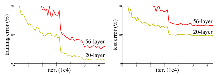
The problem of gradient vanishing on MNIST and CIFAR-10 datasets.
Researchers found that the gradient vanishing is the reason why this problem occurs. Since we use the backpropagation algorithm for training the model, we multiply the partial derivatives of the loss functions w.r.t internal operations of model. If one of the partial derivatives tends to zero, this multiplication causes the gradient to be very small and then the optimizer of the network doesn’t move in weight space. And so the model does not trained!
The Residual networks, Deep Residual Learning for Image Recognition, which are introduced by the Microsoft research team, proposes a novel technique to overcome the gradient vanishing problem. They use a skip connection between layers of the network to move the information from each layer to the next one. The layer just needs to learn a residual which helps the model to increase the classification accuracy. The next figure compares the classical networks vs. the ResNtes.
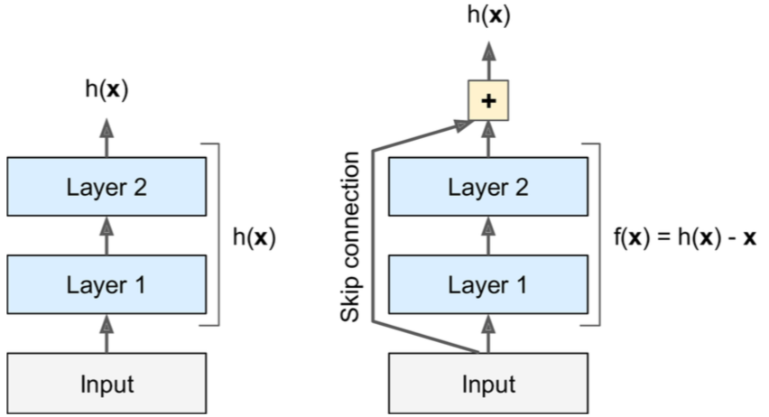
Skip connection in ResNet vs classical MLP.
The formal definition of these networks has the form
$$
\begin{aligned}
y_t &= h(z_t) + \mathcal{F}(z_t,\theta_t)\
z_{t+1} &= f(y_t)
\end{aligned}
$$
where $z_i$ is the output of $ith$ layer of the network, $\mathcal{F}$ is a block of some operations, such as single-layer non-linearity, convolutional block, etc., $\theta_i$ is the parameters of the $ith$ residual block, and $f,h$ are arbitrary functions. The function $h$ is usually set to identity mapping while $f$ maybe chose ReLU or identity. If we remove the term $h(z_t)$ this definition is equal to the classical networks. It’s worth to note that, ResNets showed a very good approximation ability on different tasks versus the classical models.
Neural ODEs
Let’s use identity mapping for both functions $f,h$ in the ResNet formulation. Then this definition reduces to
$$ z_{t+1} = z_t + \mathcal{F}(z_t, \theta_t). $$
Acutually, this definiton is very similar to the Euler method for solving ODEs! The difference is just here we set step length $\Delta t$ to $1$. More precisely, a chain of $k$ residual blocks in a neural network is the Euler method with $k$ steps where step length is set to $1$.
It seems that ResNets, which has good accuracy on different problems, solve an ODE to learn the classification task. In other words, There exists a first-order ODE which it’s solution is the best hypothesis of the task. But why we use the Euler method? why not a modern adaptive solver? Before answering the question lets look at other types of neural networks. The next table shows that there are methods that are equivalent to other ODE solvers such as backward Euler and Runge-Kutta!
| Network | Fixed-step Numerical Scheme |
|---|---|
| ResNet, RevNet, ResNeXt, etc. | Forward Euler |
| PolyNet | Approximation to Backward Euler |
| FractalNet | Runge-Kutta |
| DenseNet | Runge-Kutta |
In the formal definition, Neural ODEs try to solve this ODE to learn a pattern recognition problem:
$$ \frac{dz}{dt} = \mathcal{F}(z(t),t,\theta) $$
w.r.t initial condition $z(0) = x$ where $t \in [0, T]$ and $x$ is a sample form our dataset.
The Neural ODEs idea is to replace the Euler method with a black box ODE solver which performs much better. But this replacement has a challenge! ODE solvers evaluate the function, in the different nodes. But the ResNet model was discrete and function evaluation is applied in specific places in the domain. To do this possible, authors propose a continuous network and then replace Euler method with an modern ODE solver. The evolution of this process can be done in four phases:
- In this code snippet, a unusual kind of ResNets, we have different residual blocks, each has their parameters.
    def F(z, t, theta):
        return nnet[t](z, theta[t])

    def resnet(z):
        for t in [1:T]:
            z = z + F(z, t, theta)
        return z
- Here we have $T$ residual blocks with the same architecture while they have their own parameters. This is the most common type of ResNets.
    def F(z, t, theta):
        return nnet(z, theta[t])

    def resnet(z):
        for t in [1:T]:
            z = z + F(z, t, theta)
        return z
- Here is the idea of continuous model with shared weights. Same as the previous model, the residual blocks in this model have the same architecture and parameters. But the difference is to inputting the network by pair $[z,t]$. This model lets us call the network with the desired value $t$, not just positive integers. Based on the value $t$ the output of network changes. In this case, the for loop plays the role of Euler method ODE solver.
    def F(z, t, theta):
        return nnet([z,t], theta)

    def FixedNODE(z):
        for t in [1:T]:
            z = z + F(z, t, theta)
        return z
- Final idea: Replace the Euler method by a black box adaptive ODE solver.
    def F(z, t, theta):
        return nnet([z,t], theta)

    def AdaptiveNODE(z):
        z = ODESolve(F, z, 0, T, theta)
        return z
The next figure compares the ResNets and NODEs. You can see the effect of adaptive solver.

Left: A Residual network defines a discrete sequence of finite transformations.
Right: A ODE network defines a vector field, which continuously transforms the state.
Both: Circles represent function evaluation locations.
Till here, we proposed a continuous model and replaced the Euler method with a modern ODE solver. In other words, we replace a chain of residual blocks with an ODE-net block. The loss function can be computed with this calculation on the dataset:
$$ L(z_{T}) = L(ODESolve(\mathcal{F},z(t_0),t_0,T,\theta)) $$
The adjoint method
The next problem is how to backpropagate the error through the model and compute the gradients for the optimizer. There are two main approaches to do this. the naive approach is to backpropagate the error through the ODE solver. This approach suffers from two problems. The first is memory usage will increase much if the ODE solver uses many complex computations and the second is the numerical error caused by multiplication of partial derivatives. The next approach is a novel technique that deals with some mathematics formulations instead of just a simple backpropagation algorithm. The pros of this approach are that it does not need to track internal operations and so no need for extra memory for backpropagation, so it has $O(1)$ memory. The cons of this method are that it needs to solve an ODE for finding the gradients. The adjoint method has diffenret applications if mathematics which i will discuss it later.
Theorem 2. By defining the adjoint state
$$ a(t) = \frac{\partial L}{\partial z(t)}, $$
its dynamics are given by ODE
$$ \frac{\text{d}a(t)}{\text{d}t} = - a(t)^T \frac{\partial \mathcal{F}(z(t),t,\theta)}{\partial z} $$
Theorem 3. The gradient of the loss function w.r.t parameters, hidden states and boundary limits can be obtained by solving the augmented ODE. The following algorithm, explains the procedure proved in the previous theorem.

Properties
In this section, we recall some properties of neural ODEs.
-
The first interesting one is The dept of neural ODEs! By referring to continuous model figure, we can see that in the ResNets number of function evaluations (Black circles) are an implicit value of the number of layers. For this point of view, we use the number of function evaluations as an implicit number of layers of neural ODEs. The experiments showed that the depth of neural ODEs increases during the training phase! Increasing the number of functions evaluations, aka number of layers, means that the ODE becomes more complex and more function evaluations are needed. This maybe is a direct result of overfitting. In the augmented neural ODE section, we propose a method for reducing the number of function evaluations.
-
Another interesting fact about neural ODEs is that, if we use the adjoint method for computing gradients, we need to solve two different ODEs in the forward and backward phase. If we do this, the results showed that the function evaluations in the backward phase are about half of the number of function evaluations in the forward phase. In other words, the depth of the network in the forward phase is twice the depth of the network in the backward phase!
-
Ability of changing ODE solver’s tolerance is another property of this method. ODE solvers have methods that predict the accuracy of the solution and break the computation if the error is smaller than a tolerance. It’s obvious that by changing this tolerance, the dept of model changes. An practical technique for accelerating the model in the test time is to use a very small tolerance at the training phase and increase this to a small value on the test phase. This helps us to find the prediction in less time.
Limitations
There are some limitations in neural ODEs. The important one is the existence and uniqueness of the ODE solution. If we use usual architectures such as Convolution and LSTMs and use tanh and ReLU, the ODE has a unique solution. Another limitation is that these models are slower versus ResNets. See the original paper for other limitations.
Augmented neural ODEs
What if the map we are trying to model cannot be described by a vector field? This is the core idea of Augmented Neural ODEs paper. This figure shows a trajectory that neural ODE cannot map, but ResNet can!
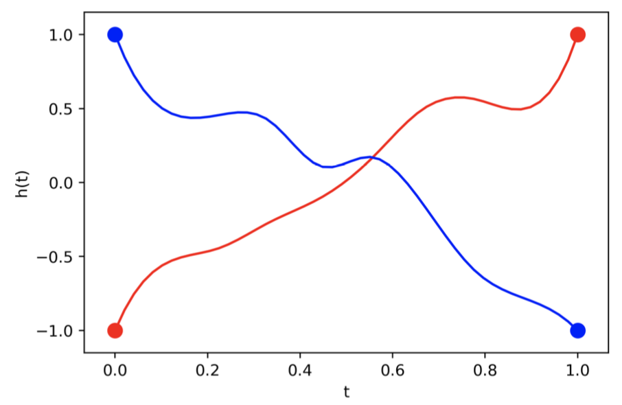


Also this figure shows that adding extra dimensions helps us to reduce the instabilities of neural ODEs.

Benchmarks
The official implementation of neural ODEs is available in the Pytorch framework. There exist non-official implementations in Tensorflow and Keras but these don’t implement the adjoint sensitivity method and so backpropagate the error through the ODE solver.
Our first test is the official architecture in mnist example of NODE. We first downsample layers. Then we use 6 connected residual blocks for feature extraction. The classification task is done by using a fully connected layer which just after an adaptive pooling layer. The residual blocks in this architecture are made by a batch normalization (BN) with ReLU activation followed by a 3x3 convolution layer with BN and ReLU activation followed by a Conv layer. For the NODE we use the same architecture by just replacing 6 residual blocks by an ODE network. The following table compares the ResNet with NODE. We also tested the NODE with and without the adjoint method. By using the adjoint method we saw that the accuracy increases a bit but the learning time increases a lot!
| Train | Test | # Params | Time | |
|---|---|---|---|---|
| ResNet | 99.56% | 99.08% | 576k | 170s |
| NODE | 99.63% | 99.05% | 208k | 615s |
| NODE+ADJ | 99.71% | 99.16% | 208k | 855s |
The big difference between ResNets and NODE is the number of parameters. The NODE uses one-third parameters versus ResNet with better accuracy. The important problem is the running time of NODE which is about 5 times slower. Also, note that using NODE needs to call 5.4k times ODE solver.
For the second example, we used the previous architecture on the Fashion MNIST dataset. We saw that same as the previous example, the NODE can reach the ResNet accuracy with much fewer parameters. The next table shows this experiment. Same as the previous experiment, the model solved 5.k ODEs to find the solution to this problem. The interesting fact is that using the adjoint method in this example not only slows down the learning time but also decreases the accuracy a bit.
| Train | Test | # Params | Time | |
|---|---|---|---|---|
| ResNet | 94.79% | 91.15% | 576k | 220s |
| NODE | 94.43% | 91.21% | 208k | 850s |
| NODE+ADJ | 93.80% | 90.81% | 208k | 1010s |