Neural ODE Tutorial
By Nadhir Hassen in Neural ODE Differential Equations Dynamical System Python
May 4, 2021
Introduction to Neural ODE
The Neural Ordinary Differential Equations paper has attracted significant attention even before it was awarded one of the Best Papers of NeurIPS 2018. The paper already gives many exciting results combining these two disparate fields, but this is only the beginning: neural networks and differential equations were born to be together. This blog post, a collaboration between authors of Flux, DifferentialEquations.jl and the Neural ODEs paper, will explain why, outline current and future directions for this work, and start to give a sense of what’s possible with state-of-the-art tools.
Rabbit population
Imagine that some rabbits make their way onto an island that doesn’t have any predators. We intially have N rabbits and after a month they make K more. After another month, those N+K rabbits make L rabbits and we observe that $\frac{N+k}{N} = \frac{L}{N+K}$, that is, the number of new-born rabbits is proportional to the number of rabbits currently on the island. If we denote time with the variable t, we’ve observed the following relationship, $$ \frac{\partial N(t)}{\partial t} = k N(t), $$ that is, the rate of change of the population is proportional to the population. You may recognise this as the continuous version of the gemoetric progression $x_n = q x_{n-1}$. This equation is simple enough such that we can solve it analytically and obtain an explicit representation of $N(t)=Ce^{kt}$ for some value $C$. Most commonly, though, it is either very difficult or impossible to find an explicit solution for an equation of this kind, for example it is unclear how to solve (if it is possible at all), $$ \left(\frac{\partial N(t)}{\partial t}\right)^3 + y^2 = N(t) y, $$ without using some advanced methods. Even if we do not knowing the exact representation, we can still do interesting things with these equations. For example, we can re-arrange and start from some initial value N(0) and (approximately) simulate how these change in time by iteratively applying the below equation for some small time difference $\Delta t$, $$ N(t \Delta t) = N(t) + \sqrt[3]{N(t) y - y^2}\Delta t. $$ This is known as the Euler method and while it doesn’t give great results due to the accumulation of errors, it shows how we can avoid requiring an explicit representation of N(t).
Making the ODE Neural
Looking at the previous section, we are inspired to ask ourselves the question what happens if we tried to model the derivative (with respect to time $t$) of the function $z(x)$ taking our inputs $x$ into our outputs $y$ with a neural network?. That is, we imagine that our function $z$ is some continuous transformation that starts at time $t=0$ at $x$ and arrives at $y$ at time $t=1$ and are interested in how it changes as we vary $t$ from 0 to 1. If we’re fitting to data anyway, we’ll learn some very complex and inscrutable function, so does it provide any advantages over trying to fit the function $z$ itself? The answer, as you may expect, is yes and we will spend the rest of this tutorial looking at various ways in which this is hepful.
Firstly, though, let’s briefly talk about exactly how we can learn the parameters $\theta$ of our network $f_{\theta}$ under this new setting. We will still employ gradient-based optimisation, which means that we need to find the quantity\n", $$ \frac{\partial L(z(1), y)}{\partial \theta} $$ where $L$ is the loss function (e.g. least squares), and $z(t)$ is the aforementioned continuous process, with $z(0) = x$ and $z(1) = \hat{y}$, that is, our prediction. Now, we know that $z(T) = z(0) + \int_0^T f_{\theta}(z(t), t) dt$, for some $0 <= T <= 1$, this is exactly us using our learnt derivative to find the value at time $t=T$ and is the analogue of running our "network" $G$ forward. Notice how we can set $T$ to be any real value, this is why we interpret Neural ODEs as having infinitely many hidden layers. As you may guess at this point, in order to fit our weights, we will need to do the equivalent of back-propagation through these infinite layers as well. This is where the concept of the adjoint state $a_z(t) = \frac{\partial L}{\partial z(t)}$ comes in - this is similar to the error signal $\delta$ in the normal neural network case. From here on out, with a bit of maths, we find the derivative of this adjoint state\n", $$ \frac{\partial a_z(t)}{\partial t} = -a_z(t)\frac{\partial f_{\theta}(z(t),t)}{\partial z(t)}. $$. Just like having the derivative of $z(t)$ allowed us to calculate $z(T)$ for any $T$, we can now calculate $a_z(T)$ as well. Note that this computation is "backwards in time" - we start from the known quantity $a(1)$ and go back towards $a(T)$. Finally, by similar argument to the above, we can define other adjoints $a_{\theta}(t)$ and $a_t(t)$ to find each of $\frac{\partial L}{\partial \theta}$ and $\frac{\partial L}{\partial t}$. Unsuprisingly, we get, $$ \frac{\partial a_{\theta}}{\partial t} = -a_z(t)\frac{\partial f_{\theta}(z(t),t)}{\partial \theta}, \\, \frac{\partial a_t}{\partial t} = -a_z(t)\frac{\partial f_{\theta}(z(t),t)}{\partial t}, $$ where again, the first line is reminiscent to how we compute the gradient of $\theta$ given the error signal $\delta$ and the current hidden state $h_t = f_{\theta}(z(t), t)$, and the last line follows the functional form of the other two. One final note is that we know $\frac{\partial L}{\partial t}$ at time $t=1$ exactly (it is $a_z(1)f_{\theta}(z(1), 1)$). With the gradients of $L$ with respect to its input parameters known, we can now minimise the function given some data.
More detail on the maths can be found in this blog post
Python Implementation
We use PyTorch to define the ODENet. We will go over the implementation from this repo as it is slightly more brief than the one in the original paper. First we modify the code as the following
def ode_solve(z0, t0, t1, f):
    """
    Simplest Euler ODE initial value solver
    """
    h_max = 0.05
    n_steps = math.ceil((abs(t1 - t0)/h_max).max().item())

    h = (t1 - t0)/n_steps
    t = t0
    z = z0

    for i_step in range(n_steps):
        z = z + h * f(z, t)
        t = t + h
    return z
We will use the following trick several times from here on. If we want to solve several ODEs (in our case one for $a_z, a_{\theta}, a_t$ each) at the same time, we can concatenate the states of each separate ODE into a single augmented state (let’s call that $a_{aug}$), and taking into account the Jacobian matrix, we can find $\frac{\partial a_{aug}(t)}{\partial t}$. This allows us to run an ODE solver on the augmented state and solve for the three variables at the same time. We define a function that performs the computation of the forward pass and the adjoint derivatives first
class ODEF(nn.Module):
    def forward_with_grad(self, z, t, grad_outputs):
        """Compute f and a df/dz, a df/dp, a df/dt"""
        batch_size = z.shape[0]

        out = self.forward(z, t)

        # a_z in the description
        a = grad_outputs
        # Computes a_z [df/dz, df/dt, df/theta] using the augmented adjoint state [a_z, a_t, a_theta]
        adfdz, adfdt, *adfdp = torch.autograd.grad(
            (out,), (z, t) + tuple(self.parameters()), grad_outputs=(a),
            allow_unused=True, retain_graph=True
        )
        # grad method automatically sums gradients for batch items, we have to expand them back
        if adfdp is not None:
            adfdp = torch.cat([p_grad.flatten() for p_grad in adfdp]).unsqueeze(0)
            adfdp = adfdp.expand(batch_size, -1) / batch_size
        if adfdt is not None:
            adfdt = adfdt.expand(batch_size, 1) / batch_size
        return out, adfdz, adfdt, adfdp

    def flatten_parameters(self):
        p_shapes = []
        flat_parameters = []
        for p in self.parameters():
            p_shapes.append(p.size())
            flat_parameters.append(p.flatten())
        return torch.cat(flat_parameters)
Next, we define a function that allows us to repeat the process described above for a series of times $[t_0, t_1, …, t_N]$. This will come in useful in the next section, where we do sequence modelling.
class ODEAdjoint(torch.autograd.Function):
    @staticmethod
    def forward(ctx, z0, t, flat_parameters, func):
        assert isinstance(func, ODEF)
        bs, *z_shape = z0.size()
        time_len = t.size(0)

        with torch.no_grad():
            z = torch.zeros(time_len, bs, *z_shape).to(z0)
            z[0] = z0
            for i_t in range(time_len - 1):
                z0 = ode_solve(z0, t[i_t], t[i_t+1], func)
                z[i_t+1] = z0

        ctx.func = func
        ctx.save_for_backward(t, z.clone(), flat_parameters)
        return z

    @staticmethod
    def backward(ctx, dLdz):
        """
        dLdz shape: time_len, batch_size, *z_shape
        """
        func = ctx.func
        t, z, flat_parameters = ctx.saved_tensors
        time_len, bs, *z_shape = z.size()
        n_dim = np.prod(z_shape)
        n_params = flat_parameters.size(0)

        # Dynamics of augmented system to be calculated backwards in time
        def augmented_dynamics(aug_z_i, t_i):
            """
            tensors here are temporal slices
            t_i - is tensor with size: bs, 1
            aug_z_i - is tensor with size: bs, n_dim*2 + n_params + 1
            """
            z_i, a = aug_z_i[:, :n_dim], aug_z_i[:, n_dim:2*n_dim]  # ignore parameters and time

            # Unflatten z and a
            z_i = z_i.view(bs, *z_shape)
            a = a.view(bs, *z_shape)
            with torch.set_grad_enabled(True):
                t_i = t_i.detach().requires_grad_(True)
                z_i = z_i.detach().requires_grad_(True)
                func_eval, adfdz, adfdt, adfdp = func.forward_with_grad(z_i, t_i, grad_outputs=a)  # bs, *z_shape
                adfdz = adfdz.to(z_i) if adfdz is not None else torch.zeros(bs, *z_shape).to(z_i)
                adfdp = adfdp.to(z_i) if adfdp is not None else torch.zeros(bs, n_params).to(z_i)
                adfdt = adfdt.to(z_i) if adfdt is not None else torch.zeros(bs, 1).to(z_i)

            # Flatten f and adfdz
            func_eval = func_eval.view(bs, n_dim)
            adfdz = adfdz.view(bs, n_dim)
            return torch.cat((func_eval, -adfdz, -adfdp, -adfdt), dim=1)

        dLdz = dLdz.view(time_len, bs, n_dim)  # flatten dLdz for convenience
        with torch.no_grad():
            ## Create placeholders for output gradients
            # Prev computed backwards adjoints to be adjusted by direct gradients
            adj_z = torch.zeros(bs, n_dim).to(dLdz)
            adj_p = torch.zeros(bs, n_params).to(dLdz)
            # In contrast to z and p we need to return gradients for all times
            adj_t = torch.zeros(time_len, bs, 1).to(dLdz)

            for i_t in range(time_len-1, 0, -1):
                z_i = z[i_t]
                t_i = t[i_t]
                f_i = func(z_i, t_i).view(bs, n_dim)

                # Compute direct gradients
                dLdz_i = dLdz[i_t]
                dLdt_i = torch.bmm(torch.transpose(dLdz_i.unsqueeze(-1), 1, 2), f_i.unsqueeze(-1))[:, 0]

                # Adjusting adjoints with direct gradients
                adj_z += dLdz_i
                adj_t[i_t] = adj_t[i_t] - dLdt_i

                # Pack augmented variable
                aug_z = torch.cat((z_i.view(bs, n_dim), adj_z, torch.zeros(bs, n_params).to(z), adj_t[i_t]), dim=-1)

                # Solve augmented system backwards
                aug_ans = ode_solve(aug_z, t_i, t[i_t-1], augmented_dynamics)

                # Unpack solved backwards augmented system
                adj_z[:] = aug_ans[:, n_dim:2*n_dim]
                adj_p[:] += aug_ans[:, 2*n_dim:2*n_dim + n_params]
                adj_t[i_t-1] = aug_ans[:, 2*n_dim + n_params:]

                del aug_z, aug_ans

            ## Adjust 0 time adjoint with direct gradients
            # Compute direct gradients
            dLdz_0 = dLdz[0]
            dLdt_0 = torch.bmm(torch.transpose(dLdz_0.unsqueeze(-1), 1, 2), f_i.unsqueeze(-1))[:, 0]

            # Adjust adjoints
            adj_z += dLdz_0
            adj_t[0] = adj_t[0] - dLdt_0
        return adj_z.view(bs, *z_shape), adj_t, adj_p, None
Finally, we define an neural network module wrapper of the function for more convenient use
class NeuralODE(nn.Module):
    def __init__(self, func):
        super(NeuralODE, self).__init__()
        assert isinstance(func, ODEF)
        self.func = func

    def forward(self, z0, t=Tensor([0., 1.]), return_whole_sequence=False):
        t = t.to(z0)
        z = ODEAdjoint.apply(z0, t, self.func.flatten_parameters(), self.func)
        if return_whole_sequence:
            return z
        else:
            return z[-1]
Continuous-time sequence models
In this section, let’s look at the first two examples:
def to_np(x):
    return x.detach().cpu().numpy()

def plot_trajectories(obs=None, times=None, trajs=None, save=None, figsize=(16, 8)):
    plt.figure(figsize=figsize)
    if obs is not None:
        if times is None:
            times = [None] * len(obs)
        for o, t in zip(obs, times):
            o, t = to_np(o), to_np(t)
            for b_i in range(o.shape[1]):
                plt.scatter(o[:, b_i, 0], o[:, b_i, 1], c=t[:, b_i, 0], cmap=cm.plasma)

    if trajs is not None:
        for z in trajs:
            z = to_np(z)
            plt.plot(z[:, 0, 0], z[:, 0, 1], lw=1.5)
        if save is not None:
            plt.savefig(save)
    plt.show()

def conduct_experiment(ode_true, ode_trained, n_steps, name, plot_freq=10):
    # Create data
    z0 = Variable(torch.Tensor([[0.6, 0.3]]))

    t_max = 6.29*5
    n_points = 200

    index_np = np.arange(0, n_points, 1, dtype=np.int)
    index_np = np.hstack([index_np[:, None]])
    times_np = np.linspace(0, t_max, num=n_points)
    times_np = np.hstack([times_np[:, None]])

    times = torch.from_numpy(times_np[:, :, None]).to(z0)
    obs = ode_true(z0, times, return_whole_sequence=True).detach()
    obs = obs + torch.randn_like(obs) * 0.01

    # Get trajectory of random timespan
    min_delta_time = 1.0
    max_delta_time = 5.0
    max_points_num = 32
    def create_batch():
        t0 = np.random.uniform(0, t_max - max_delta_time)
        t1 = t0 + np.random.uniform(min_delta_time, max_delta_time)

        idx = sorted(np.random.permutation(index_np[(times_np > t0) & (times_np < t1)])[:max_points_num])

        obs_ = obs[idx]
        ts_ = times[idx]
        return obs_, ts_

    # Train Neural ODE
    optimizer = torch.optim.Adam(ode_trained.parameters(), lr=0.01)
    for i in range(n_steps):
        obs_, ts_ = create_batch()

        z_ = ode_trained(obs_[0], ts_, return_whole_sequence=True)
        loss = F.mse_loss(z_, obs_.detach())

        optimizer.zero_grad()
        loss.backward(retain_graph=True)
        optimizer.step()

        if i % plot_freq == 0:
            z_p = ode_trained(z0, times, return_whole_sequence=True)

            plot_trajectories(obs=[obs], times=[times], trajs=[z_p], save=f"assets/imgs/{name}/{i}.png")
            clear_output(wait=True)
Simple linear ODE
We are given a two-dimensinal $\mathbf{z}(t)$, which changes according to the equation $$
\frac{\partial \mathbf{z}}{\partial t} = \begin{bmatrix}
-0.1 z_1 - z_2 \
z_1 - 0.1 z_2 \
\end{bmatrix}.
$$
This looks gives us a spiral from the initial point, going closer and closer around the origin.
# Restrict ODE to a linear function
class LinearODEF(ODEF):
    def __init__(self, W):
        super(LinearODEF, self).__init__()
        self.lin = nn.Linear(2, 2, bias=False)
        self.lin.weight = nn.Parameter(W)

    def forward(self, x, t):
        return self.lin(x)

# True function
class SpiralFunctionExample(LinearODEF):
    def __init__(self):
        super(SpiralFunctionExample, self).__init__(Tensor([[-0.1, -1.], [1., -0.1]]))

# Random initial guess for function
class RandomLinearODEF(LinearODEF):
    def __init__(self):
        super(RandomLinearODEF, self).__init__(torch.randn(2, 2)/2.)

ode_true = NeuralODE(SpiralFunctionExample())
ode_trained = NeuralODE(RandomLinearODEF())

conduct_experiment(ode_true, ode_trained, 500, "linear")
Simple linear ODE
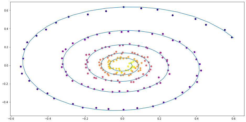
Figure 2: Spriral function with random linear ODE
More complex ODE: 2-layer neural network
Next we set up an ODE with more complicated dynamics. In this particular case, we will use a 2-layer neural network to produce the dynamics. That is, we have $$ \frac{\partial \mathbf{z}}{\partial t} = f_{true}(\mathbf{z}(t), t) $$ for some 2-layer neural network $f_{true}$.
# True 2-layer neural network
class TestODEF(ODEF):
    def __init__(self, A, B, x0):
        super(TestODEF, self).__init__()
        self.A = nn.Linear(2, 2, bias=False)
        self.A.weight = nn.Parameter(A)
        self.B = nn.Linear(2, 2, bias=False)
        self.B.weight = nn.Parameter(B)
        self.x0 = nn.Parameter(x0)

    def forward(self, x, t):
        xTx0 = torch.sum(x*self.x0, dim=1)
        dxdt = torch.sigmoid(xTx0) * self.A(x - self.x0) + torch.sigmoid(-xTx0) * self.B(x + self.x0)
        return dxdt

# Neural network to learn the dynamics
class NNODEF(ODEF):
    def __init__(self, in_dim, hid_dim, time_invariant=False):
        super(NNODEF, self).__init__()
        self.time_invariant = time_invariant

        if time_invariant:
            self.lin1 = nn.Linear(in_dim, hid_dim)
        else:
            self.lin1 = nn.Linear(in_dim+1, hid_dim)
        self.lin2 = nn.Linear(hid_dim, hid_dim)
        self.lin3 = nn.Linear(hid_dim, in_dim)
        self.elu = nn.ELU(inplace=True)

    def forward(self, x, t):
        if not self.time_invariant:
            x = torch.cat((x, t), dim=-1)

        h = self.elu(self.lin1(x))
        h = self.elu(self.lin2(h))
        out = self.lin3(h)
        return out
func = TestODEF(Tensor([[-0.1, -0.5], [0.5, -0.1]]), Tensor([[0.2, 1.], [-1, 0.2]]), Tensor([[-1., 0.]]))
ode_true = NeuralODE(func)

func = NNODEF(2, 16, time_invariant=True)
ode_trained = NeuralODE(func)

conduct_experiment(ode_true, ode_trained, 3000, "comp", plot_freq=30)
2-layer neural network
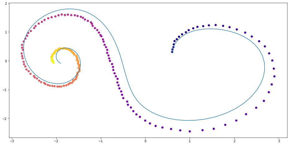
Figure 2: Spriral function with 2-layer neural network ODE
Further work
It turns out vanilla Neural ODEs are limited in what type of functions they can express. In particular, they struggle to fit functions like this because we’re working in terms of the derivative. Think about what the derivative should be at the intersection of the blue and red curve. On one hand, it needs to be positive so the blue function can increase, but on the other hand, it needs to be negative so the red line can decrease. The way to overcome this issue is to introduce some extra “ficticious” dimensions and that approach is described in the paper Augmented Neural ODEs (ANODEs). In general, it is recommended that you use ANODEs instead of vanilla NODEs. A link to the GitHub repository can be found here We here looked at only first-order ODEs (the order is the highest derivative involved in expressing the dynamics of the system). If you are interested in exploring ODEs of higher order, for example because you are interested in modelling a physical system with known dynamics that are of higher order, you can look at second-order ODEs (it briefly talks about higher orders as well), which are described here. If you are interested in making the density estimation faster and thus more scalable, it is recommended that you refer to the follow up paper Free-form Jacobian of Reversible Dynamics FFJORD. Finally, if you are interested whether this approach is extendable to Stochastic Differential Equations, you can refer to this documnet with (currently-ongoing) implementation.
- Posted on:
- May 4, 2021
- Length:
- 13 minute read, 2558 words
- Categories:
- Neural ODE Differential Equations Dynamical System Python